Connectivity

Read raw data, rest, eyes open.
View the data
Warning! cleaning data with PCA introduced false synchrony to dipoles
Read somatosensory evoked responses.
Averaging left and right responses separately
Plot left finger response
Plot right finger response
Head model
Dipole fit
Plot dipole timecourse
Now see the somatosensory cortex activation in the rest state (Mu).
Make Hilbert envelope
check correlations (don't expect much)
let's check cross correlation for absolute MEG data
now for alpha hilbert envelopes
Coherence
Another approach to left-right coherence
Compute coherence for pairs of voxels with SAMwts

Read raw data, rest, eyes open.

cd somsens
fileName='hb_c,rfhp0.1Hz';
cfg=[];
cfg.dataset=fileName;
cfg.trialdef.eventtype='TRIGGER';
cfg.trialdef.prestim=0;
cfg.trialdef.poststim=120;
cfg.trialdef.offset=0;
cfg.trialfun='BIUtrialfun';
cfg.trialdef.eventvalue= 90;
cfg.channel='MEG';
cfg=ft_definetrial(cfg);
cfg.padding=0.5;
cfg.bpfilter='yes';
cfg.bpfreq=[1 90];
cfg.demean='yes';
cfg.continuous='yes';
cfg.channel='MEG';
eyesOpen=ft_preprocessing(cfg);

evaluating trialfunction 'BIUtrialfun'
reading header...
applying digital weights in the gradiometer balancing matrix
undoing the Supine balancing
reading events from file...
applying digital weights in the gradiometer balancing matrix
undoing the Supine balancing
found 894 events
created 1 trials
the call to "ft_definetrial" took 3 seconds and an estimated 0 MB
applying digital weights in the gradiometer balancing matrix
undoing the Supine balancing
processing channel { 'A22' 'A2' 'A104' 'A241' 'A138' 'A214' 'A71' 'A26' 'A93' 'A39' 'A125' 
reading and preprocessing
reading and preprocessing trial 1 from 1
the call to "ft_preprocessing" took 5 seconds and an estimated 461 MB

View the data

see the onset of alpha for A113, A114 and A115

cfgb=[];
cfgb.layout='4D248.lay';
cfgb.continuous='yes';
cfgb.event.type='';
cfgb.event.sample=1;
cfgb.blocksize=10;
cfgb.viewmode='vertical';
cfgb.ylim=[-1e-12  1e-12];
cfgb.channel={'A112','A113','A114','A115','A116'};
comppic=ft_databrowser(cfgb,eyesOpen);

the input is raw data with 248 channels and 1 trials
detected   0 visual artifacts
redrawing with viewmode vertical
fetching data... done
fetching artifacts... done
preprocessing data... done
the call to "ft_prepare_layout" took 0 seconds and an estimated 462 MB
plotting artifacts...
plotting events...
plotting data...
done
the call to "ft_databrowser" took 7 seconds and an estimated 462 MB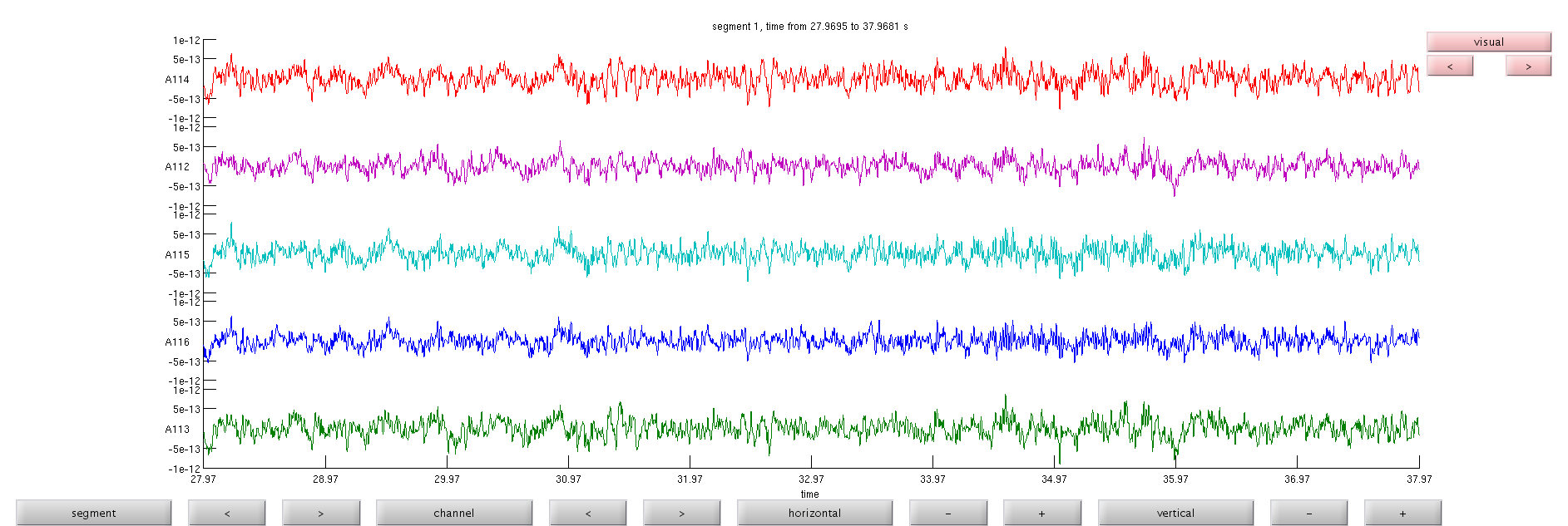

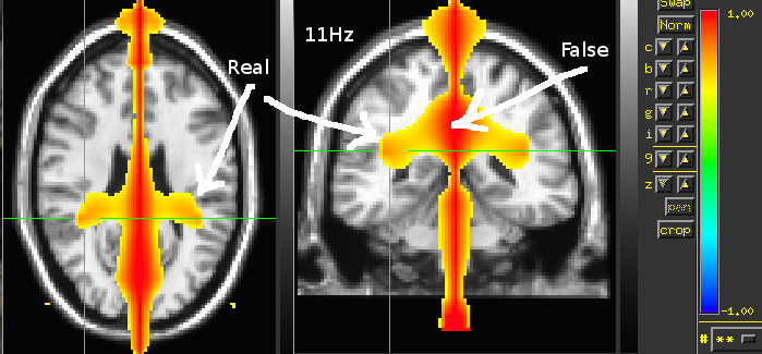
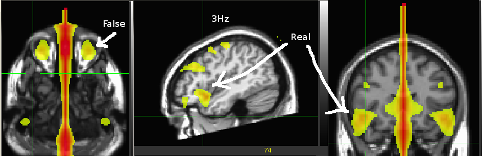
Warning! cleaning data with PCA introduced false synchrony to dipoles

do not clean artifacts with component analysis before running connectivity analysis

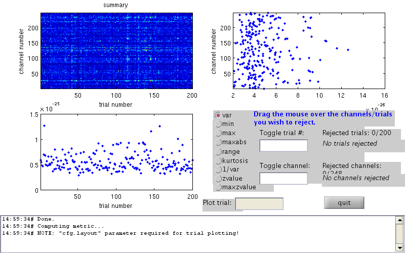
Read somatosensory evoked responses.

reject bad trials

cfg=[];
cfg.dataset=fileName;
cfg.trialdef.eventtype='TRIGGER';
cfg.trialdef.prestim=0.1;
cfg.trialdef.poststim=0.3;
cfg.trialdef.offset=-0.1;
cfg.trialfun='BIUtrialfun';
cfg.trialdef.eventvalue= [104,102]; %left index finger
cfg1=ft_definetrial(cfg);
cfg1.demean='yes';
cfg1.baselinewindow=[-0.1 0];
cfg1.bpfilter='yes';
cfg1.bpfreq=[3 30];
cfg1.channel='MEG';
cfg1.feedback='no';
somsens=ft_preprocessing(cfg1);
cfg=[];
cfg.method='summary';
cfg.channel='MEG';
cfg.alim=1e-12;
somsensCln=ft_rejectvisual(cfg, somsens);

evaluating trialfunction 'BIUtrialfun'
reading header...
applying digital weights in the gradiometer balancing matrix
undoing the Supine balancing
reading events from file...
applying digital weights in the gradiometer balancing matrix
undoing the Supine balancing
found 894 events
created 200 trials
the call to "ft_definetrial" took 3 seconds and an estimated 0 MB
applying digital weights in the gradiometer balancing matrix
undoing the Supine balancing
processing channel { 'A22' 'A2' 'A104' 'A241' 'A138' 'A214' 'A71' 'A26' 'A93' 'A39' 'A125' 'A20'
the call to "ft_preprocessing" took 6 seconds and an estimated 116 MB
the input is raw data with 248 channels and 200 trials
showing a summary of the data for all channels and trials
computing metric [--------------------------------------------------------/]
196 trials marked as GOOD, 4 trials marked as BAD
248 channels marked as GOOD, 0 channels marked as BAD
the following trials were removed: 6, 146, 157, 181
the call to "ft_rejectvisual" took 53 seconds and an estimated 1 MB

Averaging left and right responses separately

cfg=[];
cfg.feedback='no';
cfg.trials=find(somsensCln.trialinfo==102);
rightInd=ft_timelockanalysis(cfg,somsensCln);
cfg.trials=find(somsensCln.trialinfo==104);
leftInd=ft_timelockanalysis(cfg,somsensCln);

the input is raw data with 248 channels and 196 trials
selecting 99 trials
selecting 99 trials
the call to "ft_timelockanalysis" took 0 seconds and an estimated 0 MB
the input is raw data with 248 channels and 196 trials
selecting 97 trials
selecting 97 trials
the call to "ft_timelockanalysis" took 0 seconds and an estimated 0 MB

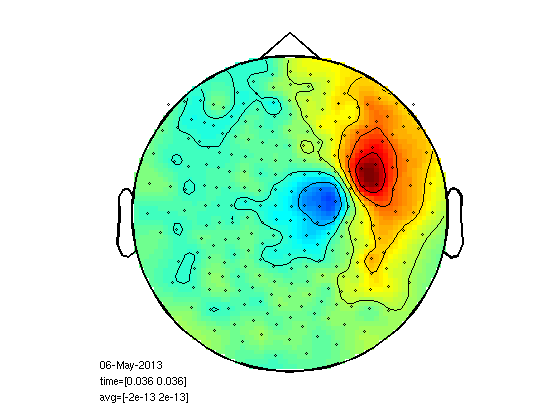
Plot left finger response

select which channels to use for dipole fit

cfg=[];
cfg.layout='4D248.lay';
cfg.interactive='yes';
cfg.zlim=[-2e-13 2e-13];
cfg.xlim=[0.036 0.036];
figure;
ft_topoplotER(cfg,leftInd);

reading layout from file 4D248.lay
the call to "ft_prepare_layout" took 0 seconds and an estimated 0 MB
the call to "ft_topoplotTFR" took 0 seconds and an estimated 0 MB
the call to "ft_topoplotER" took 0 seconds and an estimated 0 MB

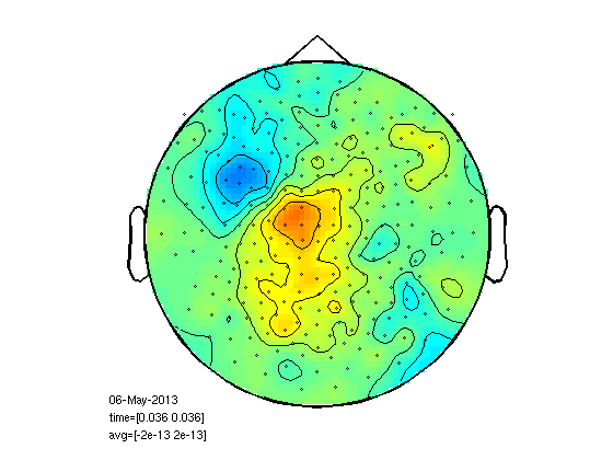
Plot right finger response

here too you have to select channels

figure;
ft_topoplotER(cfg,rightInd);

reading layout from file 4D248.lay
the call to "ft_prepare_layout" took 0 seconds and an estimated 0 MB
the call to "ft_topoplotTFR" took 0 seconds and an estimated 0 MB
the call to "ft_topoplotER" took 0 seconds and an estimated 0 MB

Head model

if exist('headmodel.mat','file')
    load headmodel
else
    [vol,grid,mesh,M1]=headmodel_BIU([],[],[],[],'localspheres');
    save headmodel vol grid mesh M1
end

Dipole fit

Here you use the channels selected at " Plot right finger response "

channelRH = {'A1', 'A2', 'A3', 'A4', 'A12', 'A13', 'A14', 'A15', 'A16', 'A17', 'A28', 'A29', 'A30', 'A31', 'A32', 'A33', 'A34', 'A35', 'A50', 'A51', 'A52', 'A53', 'A54', 'A55', 'A56', 'A57', 'A58', 'A78', 'A79', 'A80', 'A81', 'A82', 'A83', 'A84', 'A85', 'A86', 'A111', 'A112', 'A113', 'A114', 'A115', 'A116', 'A117', 'A144', 'A145', 'A146', 'A147', 'A148', 'A171', 'A172', 'A173', 'A174', 'A175', 'A193', 'A194', 'A210', 'A211'};
%channelRH = {'A11', 'A26', 'A27', 'A40', 'A41', 'A42', 'A43', 'A44', 'A45', 'A46' ... };
channelLH = {'A1', 'A2', 'A3', 'A7', 'A8', 'A9', 'A10', 'A11', 'A12', 'A21', 'A22', 'A23', 'A24', 'A25', 'A26', 'A27', 'A40', 'A41', 'A42', 'A43', 'A44', 'A45', 'A46', 'A65', 'A66', 'A67', 'A68', 'A69', 'A70', 'A71', 'A94', 'A95', 'A96', 'A97', 'A98', 'A99', 'A127', 'A128', 'A129', 'A155', 'A156', 'A157'};
t=0.0355;
cfg5 = [];
cfg5.latency = [t t];
cfg5.numdipoles = 1;
cfg5.vol=vol;
cfg5.feedback = 'textbar';
cfg5.gridsearch='yes';
cfg5.grad=ft_convert_units(leftInd.grad,'mm');
cfg5.grid=grid;
cfg5.channel=channelRH;
RHdip = ft_dipolefitting(cfg5, leftInd);
cfg5.channel=channelLH;
LHdip = ft_dipolefitting(cfg5, rightInd);
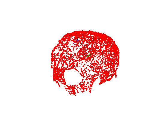
% plot dipoles
hs=ft_read_headshape('hs_file');
hs=ft_convert_units(hs,'mm');
hsx=hs.pnt(:,1);hsy=hs.pnt(:,2);hsz=hs.pnt(:,3);
figure;plot3(hsx,hsy,hsz,'r.');hold on;
ft_plot_dipole(LHdip.dip.pos,LHdip.dip.mom,'units','mm','color','b')
ft_plot_dipole(RHdip.dip.pos,RHdip.dip.mom,'units','mm','color','g')

converting units from 'm' to 'mm'
the input is timelock data with 248 channels and 407 timebins
using headmodel specified in the configuration
Your data and configuration allow for multiple sensor definitions.
Warning: using gradiometers specified in the configuration\n 
selected 57 channels
selected 1 topographies
creating dipole grid based on user specified dipole positions
3480 dipoles inside, 795 dipoles outside brain
the call to "ft_prepare_sourcemodel" took 0 seconds and an estimated 0 MB
Warning: The input units are unknown for points and S/unknown for conductivity 
scanning grid [------------------------------------------------------------]
found minimum after scanning on grid point [8.74663 -25.071 79.9769]
                                                        First-order 
 Iteration  Func-count       f(x)        Step-size       optimality
     0           4        0.0724747                        0.0021
     1          20        0.0689463            820        0.00155  
     2          28        0.0672847       0.408057        0.00155  
     3          32        0.0666039              1       0.000863  
     4          36        0.0662763              1        3.6e-05  
     5          40        0.0662757              1       7.09e-06  
     6          44        0.0662756              1        7.1e-06  
     7          48        0.0662754              1       1.74e-06  
     8          52        0.0662754              1       3.06e-07  
     9          56        0.0662754              1       7.75e-09  
    10          72        0.0662754      0.0354727       3.36e-09  

Local minimum possible.

fminunc stopped because the size of the current step is less than
the default value of the step size tolerance.



found minimum after non-linear optimization on [3.60683 -26.2694 78.6596]
the call to "ft_dipolefitting" took 8 seconds and an estimated 0 MB
the input is timelock data with 248 channels and 407 timebins
using headmodel specified in the configuration
Your data and configuration allow for multiple sensor definitions.
Warning: using gradiometers specified in the configuration\n 
selected 42 channels
selected 1 topographies
creating dipole grid based on user specified dipole positions
3480 dipoles inside, 795 dipoles outside brain
the call to "ft_prepare_sourcemodel" took 0 seconds and an estimated 0 MB
scanning grid [------------------------------------------------------------]
found minimum after scanning on grid point [9.45348 34.1831 87.5663]
                                                        First-order 
 Iteration  Func-count       f(x)        Step-size       optimality
     0           4         0.022875                       0.00155
     1          20        0.0212886            820        0.00152  
     2          24        0.0200368              1       0.000904  
     3          28        0.0195517              1       0.000273  
     4          32         0.019477              1       0.000289  
     5          36        0.0193226              1       0.000144  
     6          40        0.0193142              1          4e-05  
     7          44        0.0193134              1        6.9e-07  
     8          48        0.0193134              1       8.01e-09  
     9          52        0.0193134              1       4.05e-10  

Local minimum found.

Optimization completed because the size of the gradient is less than
the selected value of the function tolerance.



found minimum after non-linear optimization on [7.47257 37.7573 89.221]
the call to "ft_dipolefitting" took 7 seconds and an estimated 0 MB
converting units from 'm' to 'mm'

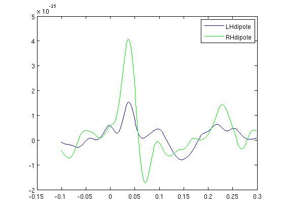
Plot dipole timecourse

cfg=[];cfg.channel=channelLH;
dataLH=ft_preprocessing(cfg,rightInd);

cfg.channel=channelRH;
dataRH=ft_preprocessing(cfg,leftInd);
timecourseLH=LHdip.dip.pot'*dataLH.avg;
timecourseRH=RHdip.dip.pot'*dataRH.avg;
figure;
plot(dataLH.time,timecourseLH,'b');
hold on;
plot(dataLH.time,timecourseRH,'g');
legend('LHdipole','RHdipole');

Warning: the trial definition in the configuration is inconsistent with the actual data 
Warning: reconstructing sampleinfo by assuming that the trials are consecutive segments of a continuous
recording 
preprocessing
preprocessing trial 1 from 1
the call to "ft_preprocessing" took 0 seconds and an estimated 0 MB
preprocessing
preprocessing trial 1 from 1
the call to "ft_preprocessing" took 0 seconds and an estimated 0 MB

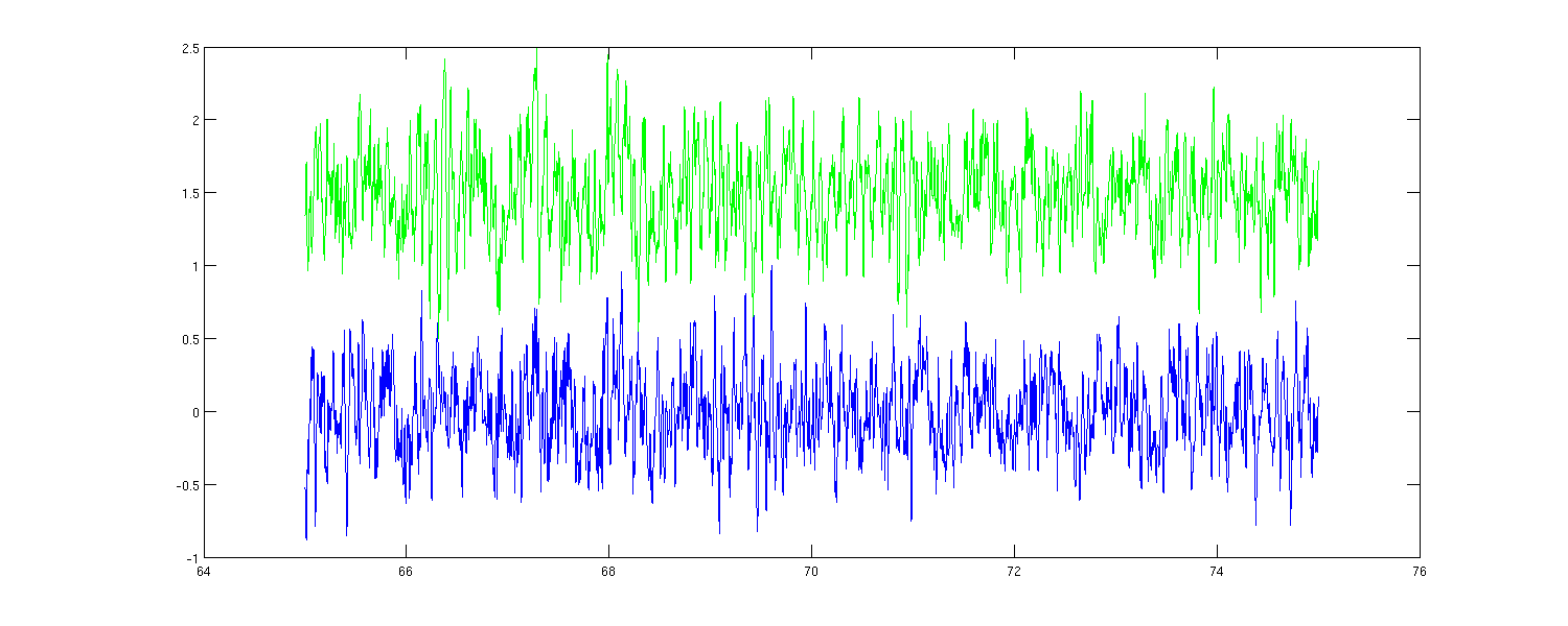
Now see the somatosensory cortex activation in the rest state (Mu).

choose channels for data display

cfg=[];cfg.channel=channelLH;
dataLH=ft_preprocessing(cfg,eyesOpen);
cfg.channel=channelRH;
dataRH=ft_preprocessing(cfg,eyesOpen);
% time window with no MOG, 65 to 75s
smp1=nearest(dataLH.time{1,1},65);
smp2=nearest(dataLH.time{1,1},75);
timecourseLH=LHdip.dip.pot'*dataLH.trial{1,1}(:,smp1:smp2);
timecourseRH=RHdip.dip.pot'*dataRH.trial{1,1}(:,smp1:smp2);
timecourseLH=timecourseLH/max(abs(timecourseLH));
timecourseRH=timecourseRH/max(abs(timecourseRH));
figure1=figure;
set(figure1,'position',[100,100,1500,600])
plot(eyesOpen.time{1,1}(:,smp1:smp2),timecourseLH,'b');
hold on;
plot(eyesOpen.time{1,1}(:,smp1:smp2),timecourseRH+1.5,'g');

preprocessing
preprocessing trial 1 from 1
the call to "ft_preprocessing" took 0 seconds and an estimated 0 MB
preprocessing
preprocessing trial 1 from 1
the call to "ft_preprocessing" took 0 seconds and an estimated 0 MB

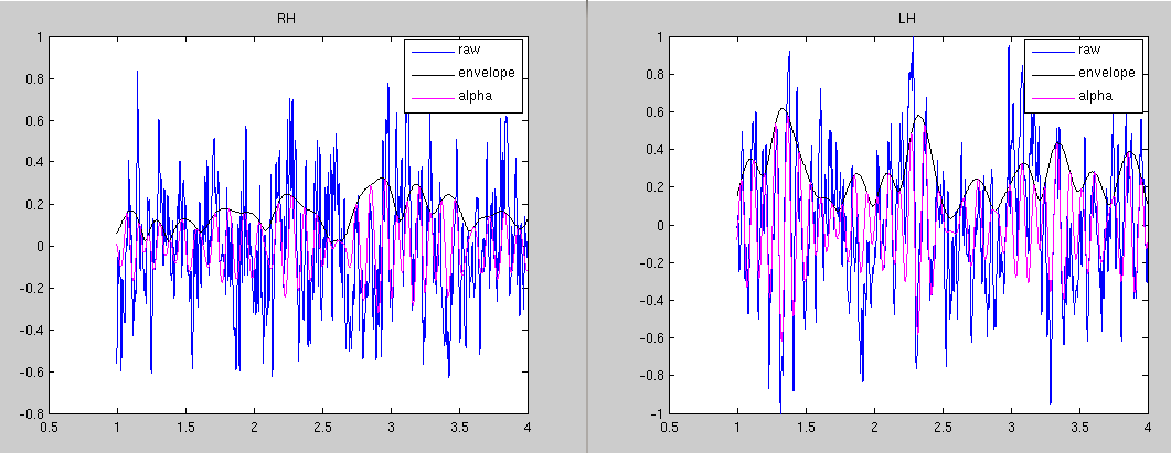
Make Hilbert envelope

vs=eyesOpen;
vs.trial{1,1}=[timecourseLH;timecourseRH];
vs.label={'Ldipole','Rdipole'};

cfg=[];
cfg.bpfilter='yes';
cfg.bpfreq=[7 13];
vsAlpha=ft_preprocessing(cfg,vs);
cfg.hilbert='yes';
vsHilb=ft_preprocessing(cfg,vs);
% plot the hilbert envelope and the data for the RH dipole
t1=1;t2=4; %sec
samp=round(1017.25.*[t1 t2])

plot(vsHilb.time{1,1}(1,samp(1):samp(2)),vs.trial{1,1}(1,samp(1):samp(2)),'b');
hold on;
plot(vsHilb.time{1,1}(1,samp(1):samp(2)),vsHilb.trial{1,1}(1,samp(1):samp(2)),'k');
plot(vsHilb.time{1,1}(1,samp(1):samp(2)),vsAlpha.trial{1,1}(1,samp(1):samp(2)),'m');
title('RH')
legend('raw','envelope','alpha')
figure; % now for the LH
plot(vsHilb.time{1,1}(1,samp(1):samp(2)),vs.trial{1,1}(2,samp(1):samp(2)),'b');
hold on;
plot(vsHilb.time{1,1}(1,samp(1):samp(2)),vsHilb.trial{1,1}(2,samp(1):samp(2)),'k');
plot(vsHilb.time{1,1}(1,samp(1):samp(2)),vsAlpha.trial{1,1}(2,samp(1):samp(2)),'m');
title('LH')
legend('raw','envelope','alpha')

preprocessing
preprocessing trial 1 from 1
the call to "ft_preprocessing" took 0 seconds and an estimated 0 MB
preprocessing
preprocessing trial 1 from 1
the call to "ft_preprocessing" took 0 seconds and an estimated 0 MB

samp =

        1017        4069

check correlations (don't expect much)

corAlpha=corrcoef(vsAlpha.trial{1,1}');corAlpha=corAlpha(1,2)
corHilb=corrcoef(vsHilb.trial{1,1}');corHilb=corHilb(1,2)
cor=corrcoef(vs.trial{1,1}');cor=cor(1,2)
corAbs=corrcoef(abs(vs.trial{1,1}'));corAbs=corAbs(1,2)

corAlpha =

   -0.1877


corHilb =

    0.0388


cor =

   -0.0507


corAbs =

    0.0353

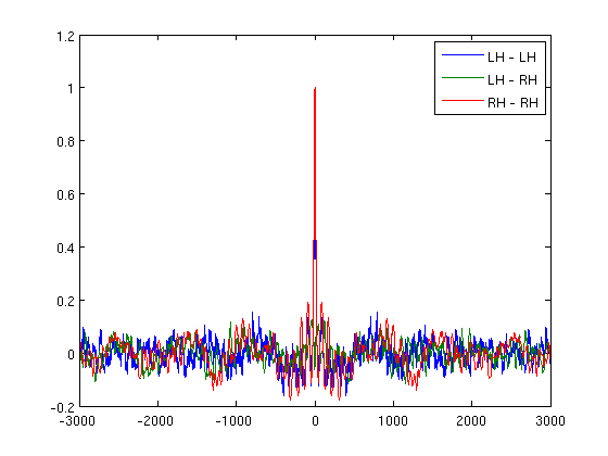
let's check cross correlation for absolute MEG data

win=3000;
[r,lags]=xcorr(vs.trial{1,1}','coeff');
sZero=find(lags==0);
figure;
plot(lags((sZero-win):(sZero+win)),r((sZero-win):(sZero+win),[1 2 4]));
legend('LH - LH','LH - RH','RH - RH')

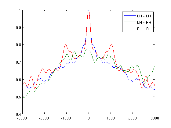
now for alpha hilbert envelopes

[r,lags]=xcorr(vsHilb.trial{1,1}','coeff');
sZero=find(lags==0);
figure;
plot(lags((sZero-win):(sZero+win)),r((sZero-win):(sZero+win),[1 2 4]));
legend('LH - LH','LH - RH','RH - RH')

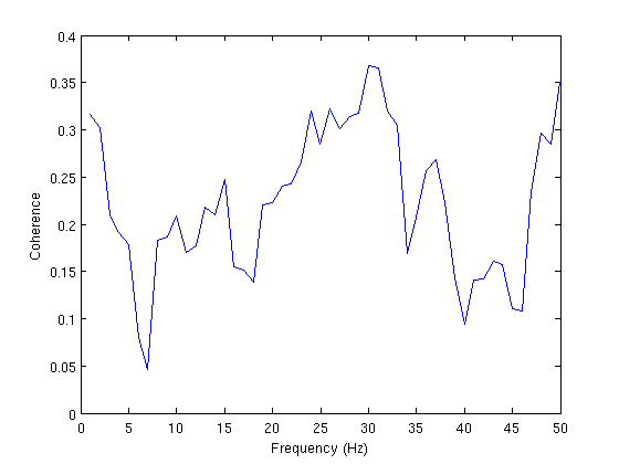
Coherence

cfg           = [];
cfg.method    = 'mtmfft';
cfg.output    = 'fourier';
cfg.tapsmofrq = 4;
cfg.foi=1:50;
freq          = ft_freqanalysis(cfg, vs);
cfg           = [];
cfg.method    = 'coh';
cohLR          = ft_connectivityanalysis(cfg, freq);
figure;
plot(cohLR.freq,squeeze(cohLR.cohspctrm(1,2,:)))
xlabel('Frequency (Hz)')
ylabel('Coherence')

the input is raw data with 2 channels and 1 trials
processing trials
processing trial 1/1 nfft: 10174 samples, datalength: 10174 samples, 79 tapers
the call to "ft_freqanalysis" took 1 seconds and an estimated 0 MB
selection fourierspctrm along dimension 2
the call to "ft_connectivityanalysis" took 0 seconds and an estimated 0 MB

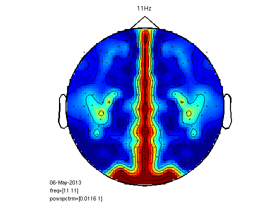
Another approach to left-right coherence

dataShort=eyesOpen;
dataShort.trial{1,1}=eyesOpen.trial{1,1}(:,smp1:smp2);
dataShort.time{1,1}=eyesOpen.time{1,1}(:,smp1:smp2);
%compute coh (not via fieldtrip) for every LR pair
temp={};
temp.label=dataShort.label;
temp.dimord='chan_freq';
temp.freq=(1:50);
temp.grad=dataShort.grad;
temp.powspctrm=ones(248,50);
coh=temp;
for cmbi=1:113
    chiL=find(strcmp(LRpairs{cmbi,1},dataShort.label));
    dataL=dataShort.trial{1,1}(chiL,:);
    chiR=find(strcmp(LRpairs{cmbi,2},dataShort.label));
    dataR=dataShort.trial{1,1}(chiR,:);
    [Cxy,F] = mscohere(dataL,dataR,[],[],[],dataShort.fsample);
    for freqi=1:50
        fi(freqi)=nearest(F,freqi); %frequency index
        coh.powspctrm(chiL,freqi)=Cxy(fi(freqi));
        coh.powspctrm(chiR,freqi)=Cxy(fi(freqi));
    end
end
cfg=[];
cfg.xlim=[11 11];
cfg.layout='4D248.lay';
figure;
ft_topoplotER(cfg,coh)
title('11Hz');
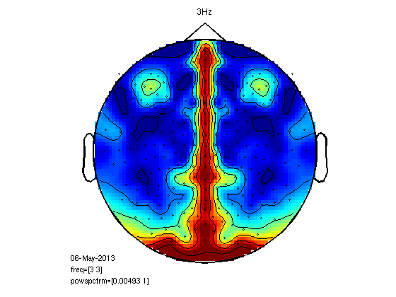
figure;
cfg.xlim=[3 3];
ft_topoplotER(cfg,coh)
title('3Hz')

reading layout from file 4D248.lay
the call to "ft_prepare_layout" took 0 seconds and an estimated 0 MB
the call to "ft_topoplotTFR" took 0 seconds and an estimated 0 MB
the call to "ft_topoplotER" took 0 seconds and an estimated 0 MB

ans = 

                 xlim: [11 11]
               layout: [1x1 struct]
          trackconfig: 'off'
          checkconfig: 'loose'
            checksize: 100000
         showcallinfo: 'yes'
                 ylim: 'maxmin'
                 zlim: 'maxmin'
                style: 'both'
            gridscale: 67
         interplimits: 'head'
        interpolation: 'v4'
           contournum: 6
             colorbar: 'no'
              shading: 'flat'
              comment: '06-May-2013
freq=[11 11]
powspctrm=[0.0116 1]'
           commentpos: 'leftbottom'
             fontsize: 8
             baseline: 'no'
               trials: 'all'
          interactive: 'no'
              hotkeys: 'no'
             renderer: []
               marker: 'on'
         markersymbol: 'o'
          markercolor: [0 0 0]
           markersize: 2
       markerfontsize: 8
            highlight: {'off'}
     highlightchannel: {{1x1 cell}}
      highlightsymbol: {'*'}
       highlightcolor: {[0 0 0]}
        highlightsize: {[6]}
    highlightfontsize: {[8]}
          labeloffset: 0.0050
        maskparameter: []
            component: []
       directionality: []
              channel: {248x1 cell}
            parameter: 'powspctrm'
             callinfo: [1x1 struct]
              version: [1x1 struct]
             previous: []

reading layout from file 4D248.lay
the call to "ft_prepare_layout" took 0 seconds and an estimated 0 MB
the call to "ft_topoplotTFR" took 0 seconds and an estimated 0 MB
the call to "ft_topoplotER" took 0 seconds and an estimated 0 MB

ans = 

                 xlim: [3 3]
               layout: [1x1 struct]
          trackconfig: 'off'
          checkconfig: 'loose'
            checksize: 100000
         showcallinfo: 'yes'
                 ylim: 'maxmin'
                 zlim: 'maxmin'
                style: 'both'
            gridscale: 67
         interplimits: 'head'
        interpolation: 'v4'
           contournum: 6
             colorbar: 'no'
              shading: 'flat'
              comment: '06-May-2013
freq=[3 3]
powspctrm=[0.00493 1]'
           commentpos: 'leftbottom'
             fontsize: 8
             baseline: 'no'
               trials: 'all'
          interactive: 'no'
              hotkeys: 'no'
             renderer: []
               marker: 'on'
         markersymbol: 'o'
          markercolor: [0 0 0]
           markersize: 2
       markerfontsize: 8
            highlight: {'off'}
     highlightchannel: {{1x1 cell}}
      highlightsymbol: {'*'}
       highlightcolor: {[0 0 0]}
        highlightsize: {[6]}
    highlightfontsize: {[8]}
          labeloffset: 0.0050
        maskparameter: []
            component: []
       directionality: []
              channel: {248x1 cell}
            parameter: 'powspctrm'
             callinfo: [1x1 struct]
              version: [1x1 struct]
             previous: []

Compute coherence for pairs of voxels with SAMwts

this requires running SAMcov and SAMwts first just watch the result in html version

% foi=11;
% [SAMHeader, ~, ActWgts]=readWeights('SAM/Raw,1-70Hz,Global.wts');
% cohlr=zeros(length(ActWgts),1);
% for Xi=-12:0.5:12
%     for Yi=-9:0.5:-0.5
%         for Zi=-2:0.5:15
%             [indR,~]=voxIndex([Xi,Yi,Zi],100.*[...
%                 SAMHeader.XStart SAMHeader.XEnd ...
%                 SAMHeader.YStart SAMHeader.YEnd ...
%                 SAMHeader.ZStart SAMHeader.ZEnd],...
%                 100.*SAMHeader.StepSize,0);
%             [indL,~]=voxIndex([Xi,-Yi,Zi],100.*[...
%                 SAMHeader.XStart SAMHeader.XEnd ...
%                 SAMHeader.YStart SAMHeader.YEnd ...
%                 SAMHeader.ZStart SAMHeader.ZEnd],...
%                 100.*SAMHeader.StepSize,0);
%             if ~isempty(find(ActWgts(indR,:))) && ~isempty(find(ActWgts(indL,:)))
%                 vsL=ActWgts(indL,:)*dataShort.trial{1,1};
%                 vsR=ActWgts(indR,:)*dataShort.trial{1,1};
%                 [Cxy,F] = mscohere(vsL,vsR,[],[],[],dataShort.fsample);
%                 fi=nearest(F,foi);
%                 cohlr(indR,1)=Cxy(fi);
%                 cohlr(indL,1)=cohlr(indR);
%                 display(['X Y Z = ',num2str([Xi,Yi,Zi])])
%             end
%         end
%     end
% end
% % plant ones in the midline
% Yi=0
% for Xi=-12:0.5:12
%     for Zi=-2:0.5:15
%         [indM,~]=voxIndex([Xi,Yi,Zi],100.*[...
%             SAMHeader.XStart SAMHeader.XEnd ...
%             SAMHeader.YStart SAMHeader.YEnd ...
%             SAMHeader.ZStart SAMHeader.ZEnd],...
%             100.*SAMHeader.StepSize,0);
%         cohlr(indM)=1;
%     end
% end
% % eval(['coh',conds{i},'=cohlr;'])
%
% cfg=[];
% cfg.step=5;
% cfg.boxSize=[-120 120 -90 90 -20 150];
% cfg.prefix='CohLR11Hz';
% VS2Brik(cfg,cohlr)