Contents

Group statistics, sensor level

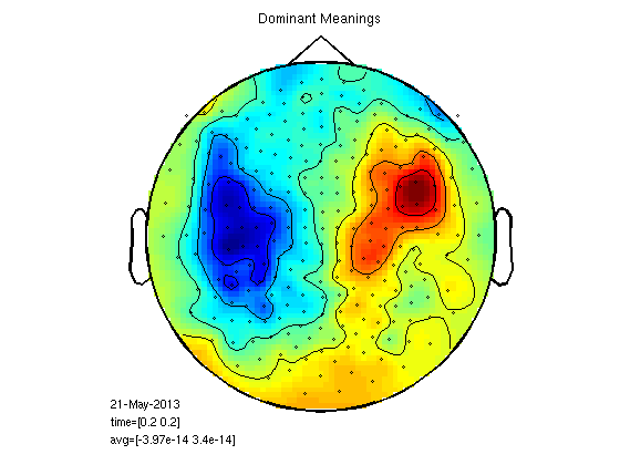
here we run sensor level statistics for reading data where biased ambiguous words were coupled with subordinate and dominant associations (see Harpaz, Lavidor and Goldstein, accepted). we found RH activity for subordinate meanings around 200ms from target word onset.

cd amb

grand average

number the average structures and make a string of names.

domstr='';
substr='';
for subi=1:25
    display(['loading subject ',num2str(subi)])
    subjn=num2str(subi);
    load ([subjn,'/DOM/dom.mat'])
    eval(['dom',subjn,'=dom;']);
    domstr=[domstr,',dom',subjn];
    load ([subjn,'/SUB/sub.mat'])
    eval(['sub',subjn,'=sub;']);
    substr=[substr,',sub',subjn];
end

cfg=[];
cfg.channel='MEG';
cfg.keepindividual = 'yes';

eval(['gadom=ft_timelockgrandaverage(cfg',domstr,');']);
eval(['gasub=ft_timelockgrandaverage(cfg',substr,');']);
clear dom* sub*

loading subject 1
loading subject 2
loading subject 3
.
.
.
loading subject 24
loading subject 25
Warning: discarding gradiometer position information because it cannot be averaged 
the call to "ft_timelockgrandaverage" took 0 seconds and an estimated 96 MB
Warning: discarding gradiometer position information because it cannot be averaged 
the call to "ft_timelockgrandaverage" took 0 seconds and an estimated 69 MB

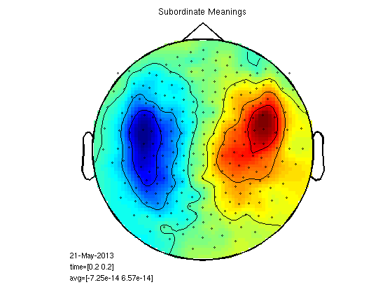
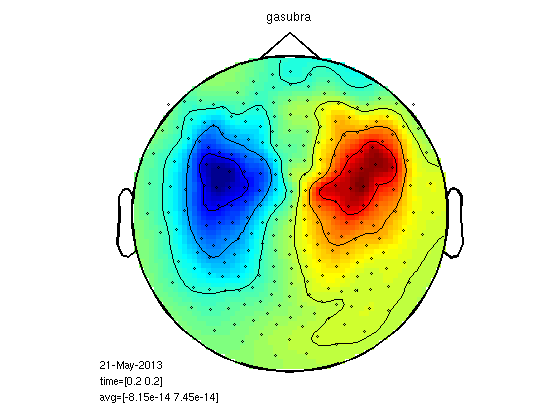
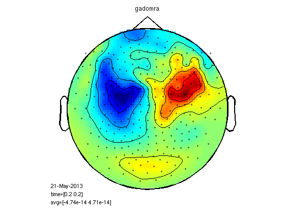
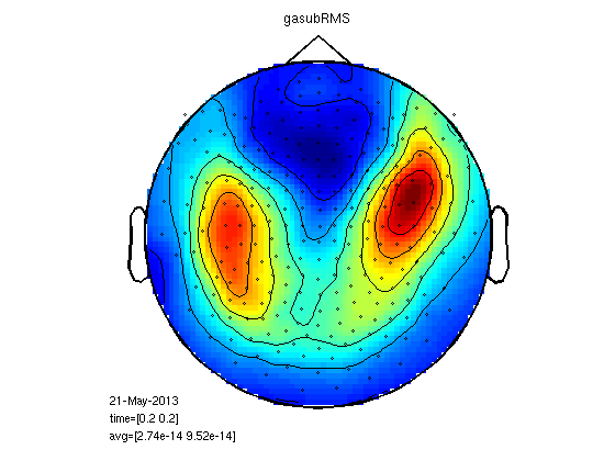
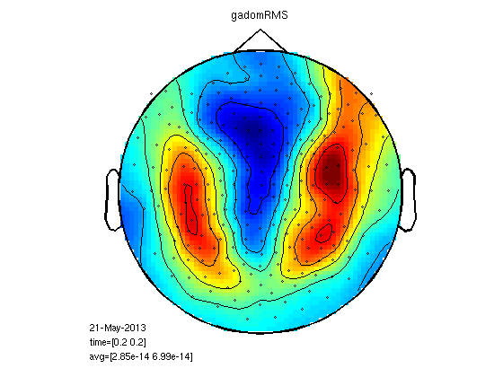
plot the fields

timepoint=0.2;
cfg=[];
cfg.zlim='maxmin';
cfg.xlim=[timepoint timepoint];
cfg.layout = '4D248.lay';
figure;
ft_topoplotER(cfg,gasub)
title ('Subordinate Meanings')
figure;
ft_topoplotER(cfg,gadom)
title ('Dominant Meanings')

the input is timelock data with 248 channels and 1017 timebins
Warning: the trial definition in the configuration is inconsistent with the actual data 
Warning: reconstructing sampleinfo by assuming that the trials are consecutive segments of a continuous
recording 
averaging trials
averaging trial 1 of 25
averaging trial 2 of 25
.
.
.
averaging trial 24 of 25
averaging trial 25 of 25
the call to "ft_timelockanalysis" took 0 seconds and an estimated 0 MB
reading layout from file 4D248.lay
the call to "ft_prepare_layout" took 0 seconds and an estimated 0 MB
the call to "ft_topoplotTFR" took 2 seconds and an estimated 69 MB
the call to "ft_topoplotER" took 2 seconds and an estimated 69 MB


time=[0.2 0.2]

the input is timelock data with 248 channels and 1017 timebins
averaging trials
averaging trial 1 of 25
.
.
.
averaging trial 25 of 25
the call to "ft_timelockanalysis" took 0 seconds and an estimated 0 MB
reading layout from file 4D248.lay
the call to "ft_prepare_layout" took 0 seconds and an estimated 0 MB
the call to "ft_topoplotTFR" took 2 seconds and an estimated 0 MB
the call to "ft_topoplotER" took 2 seconds and an estimated 0 MB

time=[0.2 0.2]

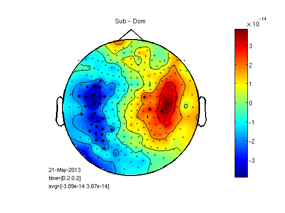
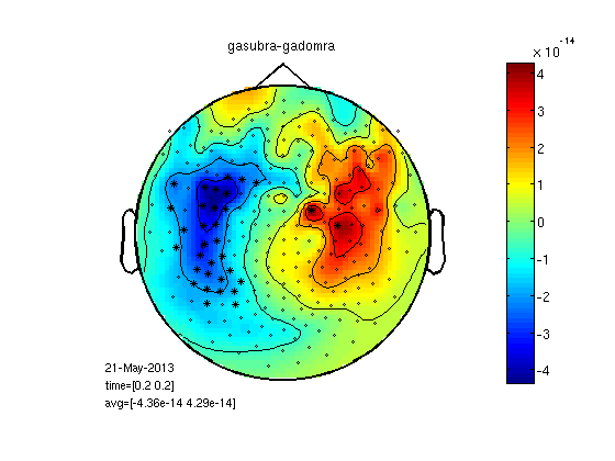
t-test per channel for one time point

cfgs=[];
cfgs.latency=[timepoint timepoint];
cfgs.method='stats';
cfgs.statistic='paired-ttest';
cfgs.design = [ones(1,25) ones(1,25)*2];
[stat] = ft_timelockstatistics(cfgs, gasub,gadom);

datadif=gadom;
datadif.individual=gasub.individual-gadom.individual;
cfg.highlight = 'on';
cfg.highlightchannel = find(stat.prob<0.05);
cfg.zlim='maxmin';
figure;ft_topoplotER(cfg, datadif);
colorbar;
title('Sub - Dom')
% I arranged the above script in a function 'statPlot11' to save space
% below. run as statPlot11(gasub,gadom,0.2)

selected 248 channels
selected 1 time bins
selected 1 frequency bins
using "statistics_stats" for the statistical testing
number of observations 248
number of replications 25 and 25
 [-----------------------------------------------------------------------/ ]
the call to "ft_timelockstatistics" took 3 seconds and an estimated 0 MB
the input is timelock data with 248 channels and 1017 timebins
averaging trials
averaging trial 1 of 25
.
.
.
averaging trial 25 of 25
the call to "ft_timelockanalysis" took 0 seconds and an estimated 0 MB
reading layout from file 4D248.lay
the call to "ft_prepare_layout" took 0 seconds and an estimated 0 MB
the call to "ft_topoplotTFR" took 2 seconds and an estimated 0 MB
the call to "ft_topoplotER" took 2 seconds and an estimated 0 MB

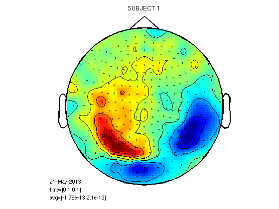
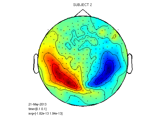
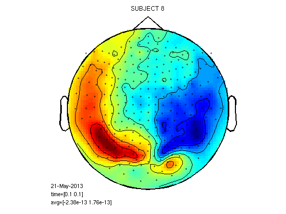
Similarity and differences between subjects in 100ms field

cfg=[];
cfg.layout='4D248.lay';
cfg.interactive='yes';
cfg.xlim=[0.1 0.1];
load 1/DOM/dom
figure;ft_topoplotER(cfg,dom);
title('SUBJECT 1')
load 2/DOM/dom
figure;ft_topoplotER(cfg,dom);
title('SUBJECT 2')
load 8/DOM/dom
figure;ft_topoplotER(cfg,dom);
title('SUBJECT 8')

reading layout from file 4D248.lay
the call to "ft_prepare_layout" took 0 seconds and an estimated 0 MB
the call to "ft_topoplotTFR" took 0 seconds and an estimated 0 MB
the call to "ft_topoplotER" took 0 seconds and an estimated 0 MB
reading layout from file 4D248.lay
the call to "ft_prepare_layout" took 0 seconds and an estimated 0 MB
the call to "ft_topoplotTFR" took 0 seconds and an estimated 0 MB
the call to "ft_topoplotER" took 0 seconds and an estimated 0 MB
reading layout from file 4D248.lay
the call to "ft_prepare_layout" took 0 seconds and an estimated 0 MB
the call to "ft_topoplotTFR" took 0 seconds and an estimated 0 MB
the call to "ft_topoplotER" took 0 seconds and an estimated 0 MB

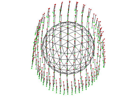
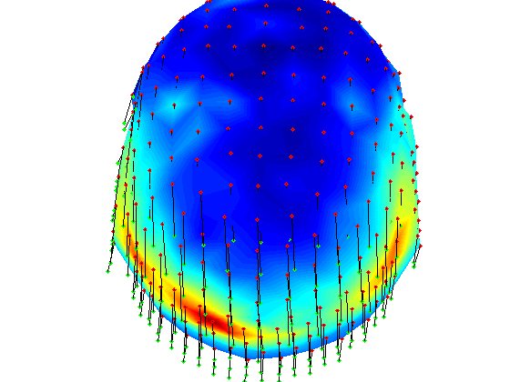
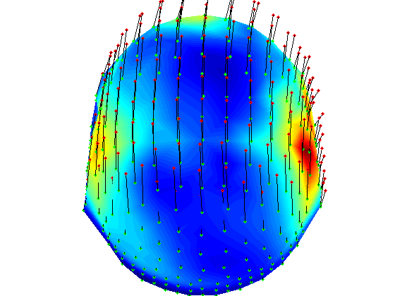
Realign subjects correct fields for head position and size

subjn='2';
load '25/DOM/dom.mat';
cfg=[];
cfg.template={dom.grad};
hs=ft_read_headshape([subjn,'/DOM/hs_file']);
[o,r]=fitsphere(hs.pnt);
load([subjn,'/DOM/dom.mat']);
cfg.inwardshift=0.025;
cfg.vol.r=r;cfg.vol.o=o;
cfg.trials=1;
dom_ra=ft_megrealign(cfg,dom);

the input is timelock data with 271 channels and 1017 timebins
selecting 1 trials
selecting 1 trials
removing 23 non-MEG channels from the data
using headmodel specified in the configuration
using gradiometers specified in the configuration
using headmodel specified in the configuration
using gradiometers specified in the configuration
mean distance towards template gradiometers is 0.03 m
creating dipole grid based on inward-shifted brain surface from volume conductor model
642 dipoles inside, 0 dipoles outside brain
the call to "ft_prepare_sourcemodel" took 0 seconds and an estimated 0 MB
computing forward model for 642 dipoles
Warning: The input units are unknown for points and S/unknown for conductivity 
pruning 149 from 248, i.e. removing the 149 smallest spatial components
computing interpolation matrix #1
computing interpolation matrix #2
computing interpolation matrix #3
pruning 146 from 248, i.e. removing the 146 smallest spatial components
realigning trial 1
original -> template             RV 53.61 %
original             -> original RV 8.71 %
original -> template -> original RV 9.80 %
Warning: showing MEG topography (RMS value over time) in the first trial only 
adding 23 non-MEG channels back to the data (MLzA, MLyA, MLzaA, MLyaA, MLxA, MLxaA, MRzA, MRxA, MRzaA, MRxaA, MRyA, MCzA, MRyaA, MCzaA, MCyA, GzxA, MCyaA, MCxA, MCxaA, GyyA, GzyA, GxxA, GyxA)
the call to "ft_megrealign" took 2 seconds and an estimated 1 MB

t-test per channel for one time point, realigned data

% here we load grandaverage files after realignment
load gadom_ra
gadomra=gadom_ra;
load gasub_ra
gasubra=gasub_ra;
% now statistics for 0.2ms
statPlot11(gasubra,gadomra,0.2)

clear *ra

the input is timelock data with 248 channels and 1017 timebins
averaging trials
averaging trial 1 of 25
.
.
.
averaging trial 25 of 25
the call to "ft_timelockanalysis" took 0 seconds and an estimated 0 MB
reading layout from file 4D248.lay
the call to "ft_prepare_layout" took 0 seconds and an estimated 0 MB
the call to "ft_topoplotTFR" took 2 seconds and an estimated 0 MB
the call to "ft_topoplotER" took 2 seconds and an estimated 0 MB
the input is timelock data with 248 channels and 1017 timebins
averaging trials
averaging trial 1 of 25
.
.
.
averaging trial 25 of 25
the call to "ft_timelockanalysis" took 0 seconds and an estimated 0 MB
reading layout from file 4D248.lay
the call to "ft_prepare_layout" took 0 seconds and an estimated 0 MB
the call to "ft_topoplotTFR" took 2 seconds and an estimated 0 MB
the call to "ft_topoplotER" took 2 seconds and an estimated 0 MB
selected 248 channels
selected 1 time bins
selected 1 frequency bins
using "statistics_stats" for the statistical testing
number of observations 248
number of replications 25 and 25
 [-----------------------------------------------------------------------/ ]
the call to "ft_timelockstatistics" took 3 seconds and an estimated 0 MB
the input is timelock data with 248 channels and 1017 timebins
averaging trials
averaging trial 1 of 25
.
.
.
averaging trial 25 of 25
the call to "ft_timelockanalysis" took 0 seconds and an estimated 0 MB
reading layout from file 4D248.lay
the call to "ft_prepare_layout" took 0 seconds and an estimated 0 MB
the call to "ft_topoplotTFR" took 2 seconds and an estimated 0 MB
the call to "ft_topoplotER" took 2 seconds and an estimated 0 MB

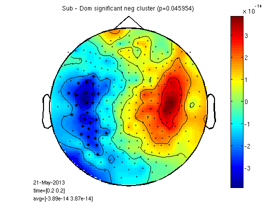
cluster based permutations statistics

Check which neghbouring channels are significantly greater / smaller for sub compared to dom. Then taking clusters of neighbours we run a permutation test to check if deviding the trials by condition is different than divide trials randomly. WHY? clustering means less comparisons, permutations means data doesn't have to be normal disyribution.

load ~/work-drafts/matlab/neighbours

%    I calculated "neighbourhood" like this:
% load '25/DOM/dom.mat';
% cfg=[];
% cfg.method='distance';
% cfg.grad=dom.grad;
% cfg.neighbourdist = 0.04; % default is 0.04m
% neighbours = ft_prepare_neighbours(cfg, dom);
% neighbours=neighbours(1:248);

cfg=[];
cfg.neighbours = neighbours;
cfg.latency     = [0.2 0.2];
cfg.numrandomization = 1000;
cfg.correctm         = 'cluster';
cfg.uvar        = 1; % row of design matrix that contains unit variable (in this case: subjects)
cfg.ivar        = 2; %
cfg.method      = 'montecarlo';
cfg.statistic   = 'depsamplesT';
cfg.design = [1:25 1:25];
cfg.design(2,:) = [ones(1,25) ones(1,25)*2];



[stat] = ft_timelockstatistics(cfg, gasub, gadom);
neg_cluster_pvals = [stat.negclusters(:).prob];
pos_cluster_pvals = [stat.posclusters(:).prob];

% realignment improve statistics? I ran:
% [stat_ra] = ft_timelockstatistics(cfg, gasub_ra, gadom_ra);
% neg_cluster_pvals = [stat_ra.negclusters(:).prob]
% pos_cluster_pvals = [stat_ra.posclusters(:).prob]
% prob was about the same

% here we select channels of significant clusters for display
neg_signif_clust = find(neg_cluster_pvals < stat.cfg.alpha);
neg = ismember(stat.negclusterslabelmat, neg_signif_clust);
%neg=ismember(neg_signif_clust,stat.negclusterslabelmat)
datadif=gasub;
datadif.individual=gasub.individual-gadom.individual;
cfgp=[];
cfgp.layout='4D248.lay';
cfgp.interactive='yes';
cfgp.xlim=[0.2 0.2];
cfgp.highlight = 'on';
cfgp.highlightchannel = find(neg);
ft_topoplotER(cfgp, datadif);colorbar;
title(['Sub - Dom significant neg cluster (p=',num2str(neg_cluster_pvals),')']);

selected 248 channels
selected 1 time bins
selected 1 frequency bins
using "statistics_montecarlo" for the statistical testing
Warning: doing a two-sided test without correcting p-values or alpha-level, p-values and alpha-level will
reflect one-sided tests per tail 
using "statfun_depsamplesT" for the single-sample statistics
constructing randomized design
total number of measurements     = 50
total number of variables        = 2
number of independent variables  = 1
number of unit variables         = 1
number of within-cell variables  = 0
number of control variables      = 0
using a permutation resampling approach
repeated measurement in variable 1 over 25 levels
number of repeated measurements in each level is 2 2 2 2 2 2 2 2 2 2 2 2 2 2 2 2 2 2 2 2 2 2 2 2 2 
computing a parametric threshold for clustering
computing statistic
estimated time per randomization is 0 seconds
computing statistic 1 from 1000
computing statistic 2 from 1000
computing statistic 3 from 1000
.
.
.
computing statistic 994 from 1000
computing statistic 995 from 1000
computing statistic 996 from 1000
computing statistic 997 from 1000
computing statistic 998 from 1000
computing statistic 999 from 1000
computing statistic 1000 from 1000
found 3 positive clusters in observed data
found 1 negative clusters in observed data
computing clusters in randomization
computing clusters in randomization 1 from 1000
.
.
.
computing clusters in randomization 997 from 1000
computing clusters in randomization 998 from 1000
computing clusters in randomization 999 from 1000
computing clusters in randomization 1000 from 1000
using a cluster-based method for multiple comparison correction
the returned probabilities and the thresholded mask are corrected for multiple comparisons
the call to "ft_timelockstatistics" took 27 seconds and an estimated 144 MB
the input is timelock data with 248 channels and 1017 timebins
averaging trials
averaging trial 1 of 25
.
.
.
averaging trial 24 of 25
averaging trial 25 of 25
the call to "ft_timelockanalysis" took 0 seconds and an estimated 0 MB
reading layout from file 4D248.lay
the call to "ft_prepare_layout" took 0 seconds and an estimated 0 MB
the call to "ft_topoplotTFR" took 2 seconds and an estimated 0 MB
the call to "ft_topoplotER" took 2 seconds and an estimated 0 MB

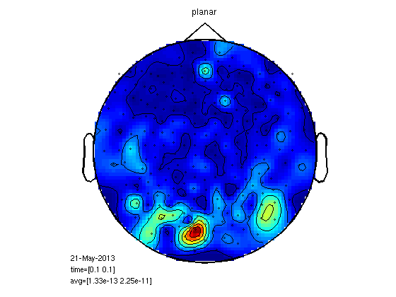
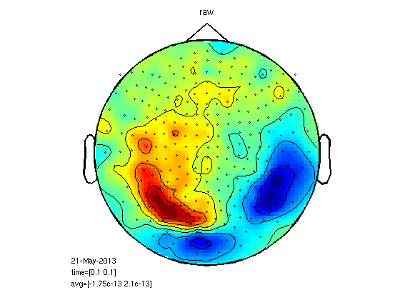
Compute planar gradient (megplanar) to reduce noise.

Relies on dipole topography. One subject, M100.

load 1/DOM/dom
cfg=[];
cfg.planarmethod   = 'orig';
cfg.neighbours     = neighbours;
[interp] = ft_megplanar(cfg, dom);
cfg=[];
cfg.combinegrad  = 'yes';
dom_cp = ft_combineplanar(cfg, interp)
cfgp = [];
cfgp.xlim=[0.1 0.1];
cfgp.layout = '4D248.lay';
figure;
ft_topoplotER(cfgp,dom_cp)
title('planar')
figure;
ft_topoplotER(cfgp,dom)
title('raw')

the input is timelock data with 271 channels and 1017 timebins
average number of neighbours is 7.85
minimum distance between neighbours is   0.02 m
maximum distance between gradiometers is   0.04 m
processing trials
processing trial 1 from 1
the call to "ft_megplanar" took 1 seconds and an estimated 0 MB
the input is timelock data with 519 channels and 1017 timebins
Warning: The field cfg.combinegrad is forbidden, it will be removed from your configuration
 
the input is timelock data with 519 channels and 1017 timebins
the input is raw data with 271 channels and 1 trials
the call to "ft_combineplanar" took 0 seconds and an estimated 0 MB


reading layout from file 4D248.lay
the call to "ft_prepare_layout" took 0 seconds and an estimated 0 MB
the call to "ft_topoplotTFR" took 0 seconds and an estimated 0 MB
the call to "ft_topoplotER" took 0 seconds and an estimated 0 MB


time=[0.1 0.1]


reading layout from file 4D248.lay
the call to "ft_prepare_layout" took 0 seconds and an estimated 0 MB
the call to "ft_topoplotTFR" took 0 seconds and an estimated 0 MB
the call to "ft_topoplotER" took 0 seconds and an estimated 0 MB


time=[0.1 0.1]

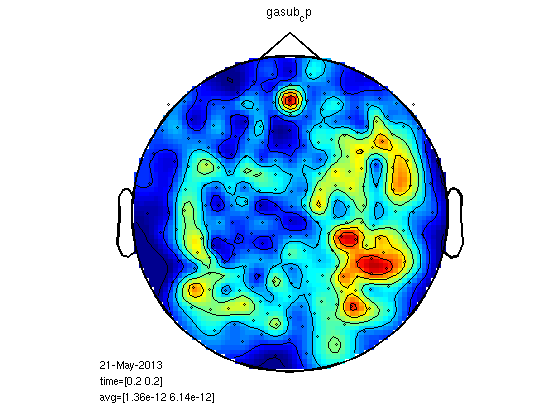
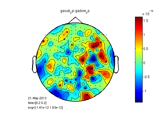
MEG planar statistics for M170

load gadom_cp
load gasub_cp

statPlot11(gasub_cp,gadom_cp,0.2)

% you can also try for M100 statPlot11(gasub_cp,gadom_cp,0.1)
% it could make sense to do megrealign after meg planar but It is
% impossible with fieldtrip now.

the input is timelock data with 248 channels and 1017 timebins
averaging trials
averaging trial 1 of 25
.
.
.
averaging trial 25 of 25
the call to "ft_timelockanalysis" took 0 seconds and an estimated 0 MB
reading layout from file 4D248.lay
the call to "ft_prepare_layout" took 0 seconds and an estimated 0 MB
the call to "ft_topoplotTFR" took 2 seconds and an estimated 0 MB
the call to "ft_topoplotER" took 2 seconds and an estimated 0 MB
the input is timelock data with 248 channels and 1017 timebins
Warning: the trial definition in the configuration is inconsistent with the actual data 
Warning: reconstructing sampleinfo by assuming that the trials are consecutive segments of a continuous
recording 
averaging trials
averaging trial 1 of 25
.
.
.
averaging trial 25 of 25
the call to "ft_timelockanalysis" took 0 seconds and an estimated 0 MB
reading layout from file 4D248.lay
the call to "ft_prepare_layout" took 0 seconds and an estimated 0 MB
the call to "ft_topoplotTFR" took 2 seconds and an estimated 0 MB
the call to "ft_topoplotER" took 2 seconds and an estimated 0 MB
selected 248 channels
selected 1 time bins
selected 1 frequency bins
using "statistics_stats" for the statistical testing
number of observations 248
number of replications 25 and 25
 [-----------------------------------------------------------------------/ ]
the call to "ft_timelockstatistics" took 3 seconds and an estimated 0 MB
the input is timelock data with 248 channels and 1017 timebins
averaging trials
averaging trial 1 of 25
.
.
.
averaging trial 25 of 25
the call to "ft_timelockanalysis" took 0 seconds and an estimated 0 MB
reading layout from file 4D248.lay
the call to "ft_prepare_layout" took 0 seconds and an estimated 0 MB
the call to "ft_topoplotTFR" took 2 seconds and an estimated 0 MB
the call to "ft_topoplotER" took 2 seconds and an estimated 0 MB

RMS for all the MEG channels

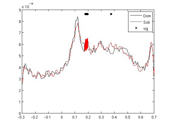
It is possible to calculate RMS for all the channels with clustData. Here we end up with one trace per condition, easy to run a ttest for each time point. We can also calculate the area between the curves.

cfg=[];
cfg.method='RMS';
cfg.neighbours='all';
gadomRMSall=clustData(cfg,gadom);
gasubRMSall=clustData(cfg,gasub);
% you can also calculate RMS without clustData in less moves:
% subRMS=squeeze(sqrt(mean(gasub.individual.^2,2)));
% domRMS=squeeze(sqrt(mean(gadom.individual.^2,2)));

cfgs=[];
cfgs.method='stats';
cfgs.statistic='paired-ttest';
cfgs.design = [ones(1,25) ones(1,25)*2];
[stat] = ft_timelockstatistics(cfgs, gasubRMSall, gadomRMSall)

plot(gadomRMSall.time,squeeze(mean(gadomRMSall.individual,1)),'k');
hold on
plot(gasubRMSall.time,squeeze(mean(gasubRMSall.individual,1)),'r');
plot(stat.time(find(stat.prob<0.05)),1.1*squeeze(max(mean(gasubRMSall.individual,1))),'k*');
legend('Dom','Sub','sig')
% don't close the figure

% area under curve
timelim=[0.17 0.2];
samp1=nearest(gadomRMSall.time,timelim(1));
samp2=nearest(gadomRMSall.time,timelim(2));
timeline=gadomRMSall.time(1,samp1:samp2);
domcurve=squeeze(gadomRMSall.individual(:,1,samp1:samp2))';
subcurve=squeeze(gasubRMSall.individual(:,1,samp1:samp2))';
domArea=trapz(timeline,domcurve);
subArea=trapz(timeline,subcurve);
[~,b]=ttest(domArea,subArea)
hsub=area(timeline,mean(subcurve,2));
set(hsub,'FaceColor','r','EdgeColor','r')
hdom=area(timeline,mean(domcurve,2));
set(hdom,'FaceColor','w','EdgeColor','w')

selected 1 channels
selected 1017 time bins
selected 1 frequency bins
using "statistics_stats" for the statistical testing
number of observations 1017
number of replications 25 and 25
 [------------------------------------------------------------------------\]
the call to "ft_timelockstatistics" took 3 seconds and an estimated 0 MB

stat = 

      mask: [1x1017 double]
      prob: [1x1017 double]
    dimord: 'chan_time'
     label: {'all'}
      time: [1x1017 double]
       cfg: [1x1 struct]


b =

    0.0130

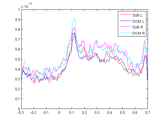
RMS for left and right sensors

cfg=[];
cfg.method='RMS';
cfg.neighbours='LR';
gadomRMS_LR=clustData(cfg,gadom);
gasubRMS_LR=clustData(cfg,gasub);

subRMS_L=squeeze(mean(gasubRMS_LR.individual(:,1,:),1));
domRMS_L=squeeze(mean(gadomRMS_LR.individual(:,1,:),1));
subRMS_R=squeeze(mean(gasubRMS_LR.individual(:,2,:),1));
domRMS_R=squeeze(mean(gadomRMS_LR.individual(:,2,:),1));

figure;
plot(gasub.time,subRMS_L,'r')
hold on
plot(gasub.time,domRMS_L,'b')
ylim([0 1e-13]);
plot(gasub.time,subRMS_R,'m')
hold on
plot(gasub.time,domRMS_R,'c')
legend('SUB L','DOM L','SUB R','DOM R')
ylim([0 1e-13]);

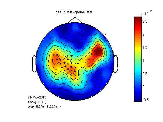
RMS for clusters

Here each channel is replaced with the RMS of its neighbours. This is good for finding why the RMS was significant over hemisphere or globally.

cfg=[];
cfg.neighbours=neighbours;
cfg.method='RMS';
gadomRMS=clustData(cfg,gadom);
gasubRMS=clustData(cfg,gasub);
statPlot11(gasubRMS,gadomRMS,0.2)

the input is timelock data with 248 channels and 1017 timebins
averaging trials
averaging trial 1 of 25
.
.
.
averaging trial 25 of 25
the call to "ft_timelockanalysis" took 0 seconds and an estimated 0 MB
reading layout from file 4D248.lay
the call to "ft_prepare_layout" took 0 seconds and an estimated 0 MB
the call to "ft_topoplotTFR" took 2 seconds and an estimated 0 MB
the call to "ft_topoplotER" took 2 seconds and an estimated 0 MB
the input is timelock data with 248 channels and 1017 timebins
averaging trials
averaging trial 1 of 25
.
.
.
averaging trial 25 of 25
the call to "ft_timelockanalysis" took 0 seconds and an estimated 0 MB
reading layout from file 4D248.lay
the call to "ft_prepare_layout" took 0 seconds and an estimated 0 MB
the call to "ft_topoplotTFR" took 2 seconds and an estimated 0 MB
the call to "ft_topoplotER" took 2 seconds and an estimated 0 MB
selected 248 channels
selected 1 time bins
selected 1 frequency bins
using "statistics_stats" for the statistical testing
number of observations 248
number of replications 25 and 25
 [-----------------------------------------------------------------------/ ]
the call to "ft_timelockstatistics" took 3 seconds and an estimated 0 MB
the input is timelock data with 248 channels and 1017 timebins
averaging trials
averaging trial 1 of 25
.
.
.
averaging trial 25 of 25
the call to "ft_timelockanalysis" took 0 seconds and an estimated 0 MB
reading layout from file 4D248.lay
the call to "ft_prepare_layout" took 0 seconds and an estimated 0 MB
the call to "ft_topoplotTFR" took 2 seconds and an estimated 0 MB
the call to "ft_topoplotER" took 2 seconds and an estimated 0 MB

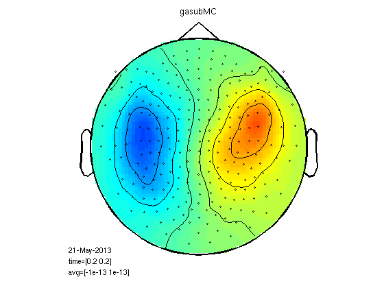
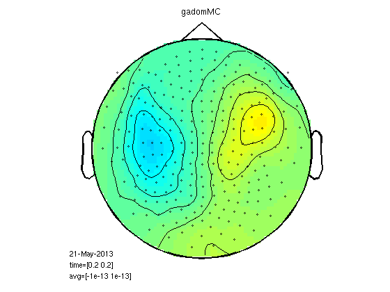
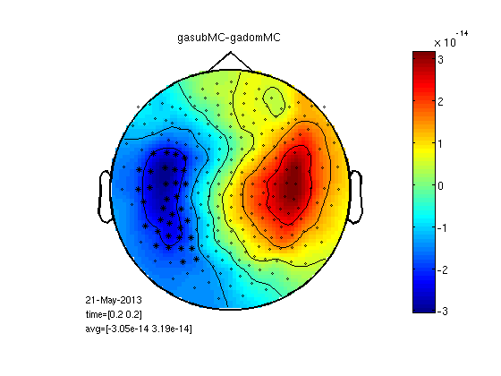
Mean cluster value

This is really smoothing of the raw signal, no RMS.

cfg.method='mean';
gadomMC=clustData(cfg,gadom);
gasubMC=clustData(cfg,gasub);
statPlot11(gasubMC,gadomMC,0.2,[-1e-13 1e-13])

the input is timelock data with 248 channels and 1017 timebins
averaging trials
averaging trial 1 of 25
.
.
.
averaging trial 25 of 25
the call to "ft_timelockanalysis" took 0 seconds and an estimated 0 MB
reading layout from file 4D248.lay
the call to "ft_prepare_layout" took 0 seconds and an estimated 0 MB
the call to "ft_topoplotTFR" took 2 seconds and an estimated 0 MB
the call to "ft_topoplotER" took 2 seconds and an estimated 0 MB
the input is timelock data with 248 channels and 1017 timebins
averaging trials
averaging trial 1 of 25
.
.
.
averaging trial 25 of 25
the call to "ft_timelockanalysis" took 0 seconds and an estimated 0 MB
reading layout from file 4D248.lay
the call to "ft_prepare_layout" took 0 seconds and an estimated 0 MB
the call to "ft_topoplotTFR" took 2 seconds and an estimated 3 MB
the call to "ft_topoplotER" took 2 seconds and an estimated 3 MB
selected 248 channels
selected 1 time bins
selected 1 frequency bins
using "statistics_stats" for the statistical testing
number of observations 248
number of replications 25 and 25
 [-----------------------------------------------------------------------/ ]
the call to "ft_timelockstatistics" took 3 seconds and an estimated 0 MB
the input is timelock data with 248 channels and 1017 timebins
averaging trials
averaging trial 1 of 25
.
.
.
averaging trial 25 of 25
the call to "ft_timelockanalysis" took 0 seconds and an estimated 0 MB
reading layout from file 4D248.lay
the call to "ft_prepare_layout" took 0 seconds and an estimated 0 MB
the call to "ft_topoplotTFR" took 2 seconds and an estimated 0 MB
the call to "ft_topoplotER" took 2 seconds and an estimated 0 MB

Published with MATLAB® 7.11