Frequency and Time Frequency analysis

Here we do frequency analysis to visual data. We first reject trials with high frequency noise (muscles). Next we correct MOG (eye movement artifact). After cleaning we perform frequency analysis and then time frequency analysis. The data we use is already after heartbeat correction.

Reject high frequency noise trials (muscle artifact)
Clean MOG by PCA, find Up-Down component
Clean MOG by PCA, find L-R component
Now you clean the data of MOG
Check if there are bad trials left
Frequency analysis
Time-Frequency analysis
Window size effect
3 cycles per windows
7 cycles per windows
1 cycle, all channels
Normalization
Within subject (between trials) statistics.

reject high frequency noise trials (muscle artifact)

here we read the data with a 60Hz high pass filter we take a large window because of the sliding windows for low freqs

cd somsens

fileName='hb_c,rfhp0.1Hz';
cfg=[];
cfg.dataset=fileName;
cfg.trialdef.eventtype='TRIGGER';
cfg.trialdef.prestim=0.5;
cfg.trialdef.poststim=1;
cfg.trialdef.offset=-0.5; %NOTE large baseline to measure low freq
cfg.trialdef.visualtrig= 'visafter';
cfg.trialfun='BIUtrialfun';
cfg.trialdef.eventvalue= [222 230 240 250];
cfg=ft_definetrial(cfg);

cfg.demean='yes';
cfg.baselinewindow=[-0.5 0];
cfg.channel='MEG';
cfg.padding=0.1;
cfg.feedback='no';
dataorig=ft_preprocessing(cfg);

cfg=[];
cfg.method='summary';
cfg.channel='MEG';
cfg.alim=1e-12;
cfg1.hpfilter='yes';
cfg1.hpfreq=60; %SEE?
dataNoMscl=ft_rejectvisual(cfg, dataorig); % data high freq reject visual
% reject bad trials

evaluating trialfunction 'BIUtrialfun'
reading header...
applying digital weights in the gradiometer balancing matrix
undoing the Supine balancing
reading events from file...
applying digital weights in the gradiometer balancing matrix
undoing the Supine balancing
found 894 events
created 160 trials
the call to "ft_definetrial" took 3 seconds and an estimated 0 MB
applying digital weights in the gradiometer balancing matrix
undoing the Supine balancing
processing channel { 'A22' 'A2' 'A104' 'A241' 'A138' 'A214' 'A71' 'A26' 'A93' 'A39' 'A125' 'A20' 'A65' 'A9' 'A8' 'A95' 'A114' 'A175' 'A16' 'A228' 'A35' 'A191' 'A37' 'A170' 'A207' 'A112' 'A224' 'A82' 'A238' 'A202' 'A220' 'A28' 'A239' 'A13' 'A165' 'A204' 'A233' 'A98' 'A25' 'A70' 'A72' 'A11' 'A47' 'A160' 'A64' 'A3' 'A177' 'A63' 'A155' 'A10' 'A127' 'A67' 'A115' 'A247' 'A174' 'A194' 'A5' 'A242' 'A176' 'A78' 'A168' 'A31' 'A223' 'A245' 'A219' 'A12' 'A186' 'A105' 'A222' 'A76' 'A50' 'A188' 'A231' 'A45' 'A180' 'A99' 'A234' 'A215' 'A235' 'A181' 'A38' 'A230' 'A91' 'A212' 'A24' 'A66' 'A42' 'A96' 'A57' 'A86' 'A56' 'A116' 'A151' 'A141' 'A120' 'A189' 'A80' 'A210' 'A143' 'A113' 'A27' 'A137' 'A135' 'A167' 'A75' 'A240' 'A206' 'A107' 'A130' 'A100' 'A43' 'A200' 'A102' 'A132' 'A183' 'A199' 'A122' 'A19' 'A62' 'A21' 'A229' 'A84' 'A213' 'A55' 'A32' 'A85' 'A146' 'A58' 'A60' 'A88' 'A79' 'A169' 'A54' 'A203' 'A145' 'A103' 'A163' 'A139' 'A49' 'A166' 'A156' 'A128' 'A68' 'A159' 'A236' 'A161' 'A121' 'A4' 'A61' 'A6' 'A126' 'A14' 'A94' 'A15' 'A193' 'A150' 'A227' 'A59' 'A36' 'A225' 'A195' 'A30' 'A109' 'A172' 'A108' 'A81' 'A171' 'A218' 'A173' 'A201' 'A74' 'A29' 'A164' 'A205' 'A232' 'A69' 'A157' 'A97' 'A217' 'A101' 'A124' 'A40' 'A123' 'A153' 'A178' 'A1' 'A179' 'A33' 'A147' 'A117' 'A148' 'A87' 'A89' 'A243' 'A119' 'A52' 'A142' 'A211' 'A190' 'A53' 'A192' 'A73' 'A226' 'A136' 'A184' 'A51' 'A237' 'A77' 'A129' 'A131' 'A198' 'A197' 'A182' 'A46' 'A92' 'A41' 'A90' 'A7' 'A23' 'A83' 'A154' 'A34' 'A17' 'A18' 'A248' 'A149' 'A118' 'A208' 'A152' 'A140' 'A144' 'A209' 'A110' 'A111' 'A244' 'A185' 'A246' 'A162' 'A106' 'A187' 'A48' 'A221' 'A196' 'A133' 'A158' 'A44' 'A134' 'A216' }
the call to "ft_preprocessing" took 5 seconds and an estimated 0 MB
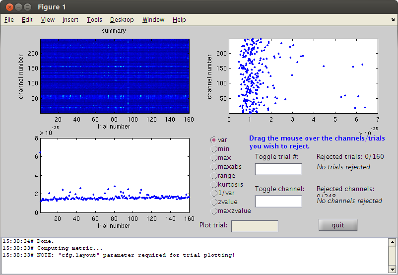
the input is raw data with 248 channels and 160 trials
showing a summary of the data for all channels and trials
computing metric [--------------------------------------------------------\]
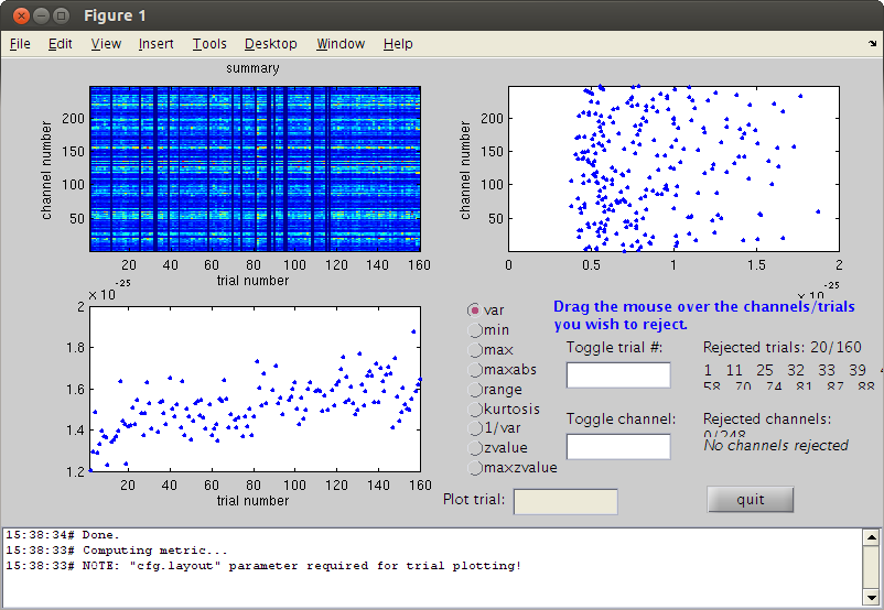
145 trials marked as GOOD, 15 trials marked as BAD
248 channels marked as GOOD, 0 channels marked as BAD
the following trials were removed: 1, 11, 25, 33, 39, 44, 70, 74, 81, 87, 90, 95, 108, 109, 115
the call to "ft_rejectvisual" took 11 seconds and an estimated 0 MB

clean MOG by PCA, find Up-Down component

first clear some memory

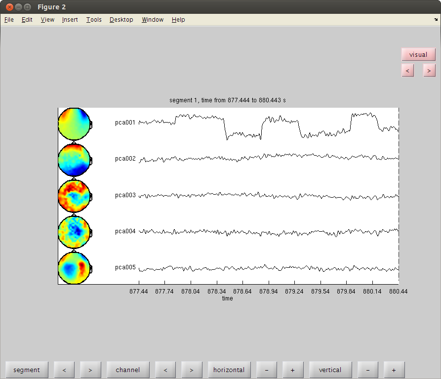
clear dataorig

trig=readTrig_BIU(fileName);
trig=clearTrig(trig);
% up-down eye movement
startt=find(trig==50,1)/1017.25; %877.4451
endt=find(trig==52,1)/1017.25; %886.3406
cfg2=[];
cfg2.dataset=fileName;
cfg2.trialdef.beginning=startt;
cfg2.trialdef.end=endt;
cfg2.trialfun='trialfun_raw'; % the other usefull trialfun we have are trialfun_beg and trialfun_BIU
cfg=ft_definetrial(cfg2);
cfg.demean='yes';% old version was: cfg1.blc='yes';
%cfg1.baselinewindow=[-0.1,0];
cfg.lpfilter='yes';
cfg.lpfreq=40;
cfg.channel='MEG';
MOGud=ft_preprocessing(cfg);
% left right eye movement
startt=find(trig==52,1)/1017.25;
endt=find(trig==54,1)/1017.25;
cfg2.trialdef.beginning=startt;
cfg2.trialdef.end=endt;
cfg=ft_definetrial(cfg2);
cfg.demean='yes';% old version was: cfg1.blc='yes';
%cfg1.baselinewindow=[-0.1,0];
cfg.lpfilter='yes';
cfg.lpfreq=40;
cfg.channel='MEG';
cfg.feedback='no';
MOGlr=ft_preprocessing(cfg);

cfg=[];
cfg.method='pca';
compMOGud           = ft_componentanalysis(cfg, MOGud);
compMOGlr           = ft_componentanalysis(cfg, MOGlr);
% see the components and find the HB and MOG artifact
% remember the numbers of the bad components and close the data browser
cfg=[];
cfg.layout='4D248.lay';
cfg.channel = 1:5;
cfg.continuous='yes';
cfg.event.type='';
cfg.event.sample=1;
cfg.blocksize=3;
ft_databrowser(cfg,compMOGud);

close

Warning: 50Hz cleaning with cleanMEG pack will not be possible using the new trigger
evaluating trialfunction 'trialfun_raw'
reading header...
Warning: READ_HEADER is only a compatibility wrapper, which will soon be removed. Please instead
call FT_READ_HEADER.
applying digital weights in the gradiometer balancing matrix
undoing the Supine balancing
found 1 events
created 1 trials
the call to "ft_definetrial" took 1 seconds and an estimated 0 MB
applying digital weights in the gradiometer balancing matrix
undoing the Supine balancing
processing channel { 'A22' 'A2' 'A104' 'A241' 'A138' 'A214' 'A71' 'A26' 'A93'
reading and preprocessing
reading and preprocessing trial 1 from 1
the call to "ft_preprocessing" took 1 seconds and an estimated 0 MB
evaluating trialfunction 'trialfun_raw'
reading header...
Warning: READ_HEADER is only a compatibility wrapper, which will soon be removed. Please instead
call FT_READ_HEADER.
applying digital weights in the gradiometer balancing matrix
undoing the Supine balancing
found 1 events
created 1 trials
the call to "ft_definetrial" took 1 seconds and an estimated 0 MB
applying digital weights in the gradiometer balancing matrix
undoing the Supine balancing
processing channel { 'A22' 'A2' 'A104' 'A241' 'A138' 'A214' 'A71' 'A26' 'A93'
the call to "ft_preprocessing" took 1 seconds and an estimated 0 MB
the input is raw data with 248 channels and 1 trials
selecting 248 channels
baseline correcting data
scaling data with 1 over 0.000000
concatenating data.
concatenated data matrix size 248x9050
starting decomposition using pca
applying the mixing matrix to the sensor description
the call to "ft_componentanalysis" took 0 seconds and an estimated 0 MB
the input is raw data with 248 channels and 1 trials
selecting 248 channels
baseline correcting data
scaling data with 1 over 0.000000
concatenating data.
concatenated data matrix size 248x11287
starting decomposition using pca
applying the mixing matrix to the sensor description
the call to "ft_componentanalysis" took 0 seconds and an estimated 0 MB
reading layout from file 4D248.lay
the call to "ft_prepare_layout" took 1 seconds and an estimated 0 MB
the input is component data with 248 components and 248 original channels
detected 0 visual artifacts
redrawing with viewmode component
fetching data... done
fetching artifacts... done
preprocessing data... done
the call to "ft_prepare_layout" took 0 seconds and an estimated 0 MB
plotting artifacts...
plotting events...
plotting data...
the call to "ft_prepare_layout" took 0 seconds and an estimated 0 MB
plotting component topographies...
done

clean MOG by PCA, find L-R component

ft_databrowser(cfg,compMOGlr);
% remember the component number for up-down and for left-right MOG. we'll
close

reading layout from file 4D248.lay
the call to "ft_prepare_layout" took 1 seconds and an estimated 0 MB
the input is component data with 248 components and 248 original channels
detected   0 visual artifacts
redrawing with viewmode component
fetching data... done
fetching artifacts... done
preprocessing data... done
the call to "ft_prepare_layout" took 0 seconds and an estimated 0 MB
plotting artifacts...
plotting events...
plotting data...
the call to "ft_prepare_layout" took 0 seconds and an estimated 0 MB
plotting component topographies...
done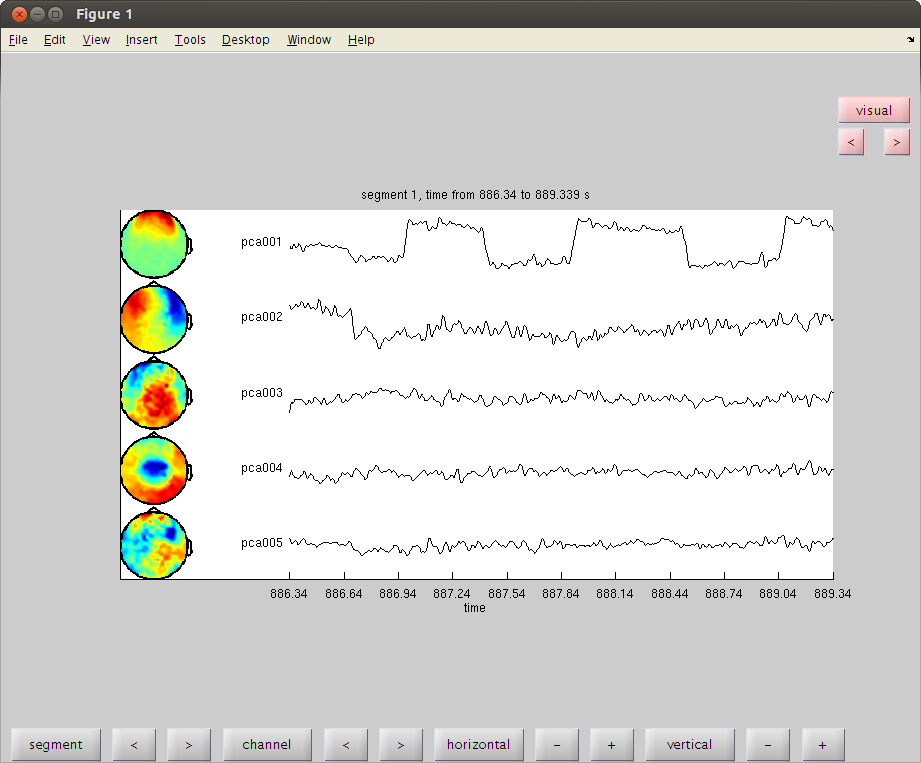

now you clean the data of MOG

set the bad comps as the value for cfgrc.component.

cfg = [];
cfg.component = 1; % change
cfg.feedback='no';
dataca = ft_rejectcomponent(cfg, compMOGud,dataNoMscl);
cfg.component = 1; % change
dataca = ft_rejectcomponent(cfg, compMOGlr,dataca);
% clear the workspace a little.
clear dataNoMscl comp* MOG* trig cfg* endt startt

baseline correcting data 
removing 1 components
keeping 247 components
the call to "ft_rejectcomponent" took 9 seconds and an estimated 0 MB
baseline correcting data 
removing 1 components
keeping 247 components
the call to "ft_rejectcomponent" took 8 seconds and an estimated 0 MB

check if there are bad trials left

cfg=[];
cfg.method='summary'; %trial
cfg.channel='MEG';
cfg.alim=1e-12;
datacln=ft_rejectvisual(cfg, dataca);
clear dataca

the input is raw data with 248 channels and 145 trials
showing a summary of the data for all channels and trials
computing metric [--------------------------------------------------------\]
144 trials marked as GOOD, 1 trials marked as BAD
248 channels marked as GOOD, 0 channels marked as BAD
the following trials were removed: 52
the call to "ft_rejectvisual" took 10 seconds and an estimated 0 MB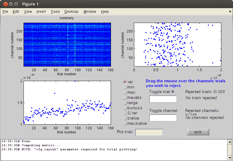

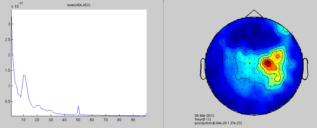
frequency analysis

cfgfr=[];
%cfgfr.trials=find(datacln.trialinfo==222);
cfgfr.output       = 'pow';
cfgfr.channel      = 'MEG';
cfgfr.method       = 'mtmfft';
cfgfr.taper        = 'hanning';
cfgfr.foi          = 1:100;
cfgfr.feedback='no';
FrAll = ft_freqanalysis(cfgfr, datacln);

% plot results for alpha
cfgp = [];
cfgp.xlim = [9 11];
cfgp.layout       = '4D248.lay';
cfgp.interactive='yes';
ft_topoplotER(cfgp, FrAll);

the call to "ft_freqanalysis" took 3 seconds and an estimated 0 MB
reading layout from file 4D248.lay
the call to "ft_prepare_layout" took 0 seconds and an estimated 0 MB
Warning: Some points fall outside the outline, please consider using another layout 
the call to "ft_topoplotTFR" took 0 seconds and an estimated 0 MB
the call to "ft_topoplotER" took 0 seconds and an estimated 0 MB

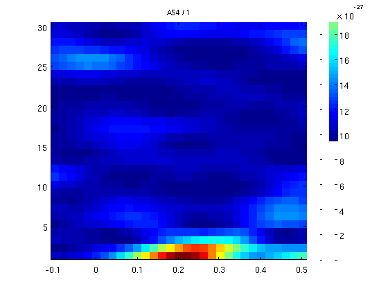
time-frequency analysis

% go to FieldTrip website and search for time frequency tutorial

% we will check frequencies with a moving window of 0.5s. the freq
% resolution is therefore 2Hz (1/winlength).
% we set the window size in the field t_ftimwin
% just to play with it a little we test only trial number 1.
cfgtfr              = [];
cfgtfr.output       = 'pow';
cfgtfr.channel      = 'MEG';
cfgtfr.method       = 'mtmconvol';
cfgtfr.taper        = 'hanning';
cfgtfr.foi          = 1:30;                            % freq of interest 3 to 100Hz
cfgtfr.t_ftimwin    = ones(length(cfgtfr.foi),1).*0.5;  % length of time window fixed at 0.5 sec
cfgtfr.toi          = -0.1:0.02:0.5;                    % time window "slides" from -0.1 to 0.5 sec in steps of 0.02 sec (20 ms)
cfgtfr.trials=1;
cfgtfr.channel='A54';
cfgtfr.feedback='no';
TFtest = ft_freqanalysis(cfgtfr, datacln);
% now plot one channel
figure;ft_singleplotTFR([], TFtest);

selecting 1 trials
selecting 1 trials
the call to "ft_freqanalysis" took 0 seconds and an estimated 0 MB
the call to "ft_singleplotTFR" took 0 seconds and an estimated 0 MB

Window size effect

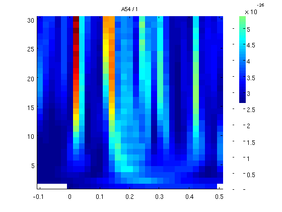
now a window with smaller size for smaller frequencies we start with a window length of 1 cycle for every frequency

cfgtfr.t_ftimwin    = 1./cfgtfr.foi;  % 1 cycle per window
TFtest = ft_freqanalysis(cfgtfr, datacln);
figure;ft_singleplotTFR([], TFtest);

selecting 1 trials
selecting 1 trials
the call to "ft_freqanalysis" took 0 seconds and an estimated 0 MB
the call to "ft_singleplotTFR" took 0 seconds and an estimated 0 MB

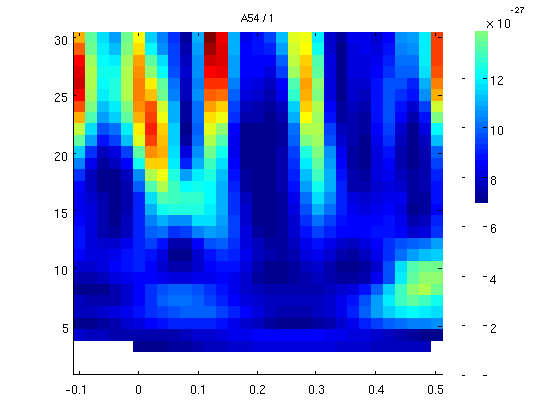
3 cycles per windows

we now move to 3 cycles per window (10Hz will be tested with a sliding window of 30ms. more cycles - smoother results but you loose low freqs.

cfgtfr.t_ftimwin    = 3./cfgtfr.foi;  % 1 cycle per window
TFtest = ft_freqanalysis(cfgtfr, datacln);
figure;ft_singleplotTFR([], TFtest);

selecting 1 trials
selecting 1 trials
the call to "ft_freqanalysis" took 0 seconds and an estimated 0 MB
the call to "ft_singleplotTFR" took 0 seconds and an estimated 0 MB

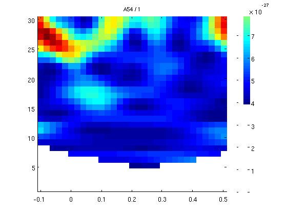
7 cycles per windows

cfgtfr.t_ftimwin    = 7./cfgtfr.foi;  % 1 cycle per window
TFtest = ft_freqanalysis(cfgtfr, datacln);
figure;ft_singleplotTFR([], TFtest);

selecting 1 trials
selecting 1 trials
the call to "ft_freqanalysis" took 0 seconds and an estimated 0 MB
the call to "ft_singleplotTFR" took 0 seconds and an estimated 0 MB

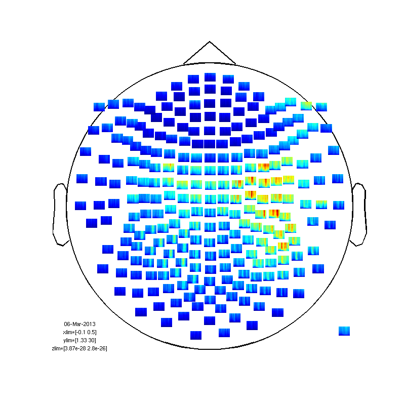
1 cycle, all channels

now we'll do 1 cycle per freq for the whole data and all the channels. it will take a few minutes.

cfgtfr.t_ftimwin    = 1./cfgtfr.foi;
cfgtfr.trials='all';
cfgtfr.channel='MEG';
cfgtfr.keeptrials='yes';
TFrAll = ft_freqanalysis(cfgtfr, datacln);
cfgp = [];
%cfgp.ylim = [3 30];
fig1=figure;
set(fig1,'Position',[0,0,800,800]);
cfgp.layout       = '4D248.lay';
cfgp.interactive='yes';
ft_multiplotTFR(cfgp, TFrAll);

the call to "ft_freqanalysis" took 77 seconds and an estimated 253 MB
the input is freq data with 248 channels, 30 frequencybins and 31 timebins
the call to "ft_freqdescriptives" took 0 seconds and an estimated 252 MB
reading layout from file 4D248.lay
the call to "ft_prepare_layout" took 0 seconds and an estimated 252 MB
Warning: (one of the) axis is/are not evenly spaced, but plots are made as if axis are linear 
the call to "ft_multiplotTFR" took 1 seconds and an estimated 252 MB

Normalization

a bit messy. needs some normalization.

fig2=figure;
set(fig2,'Position',[0,0,800,800]);
cfgp.baseline=[-0.5 0];
cfgp.baselinetype = 'relative'; %or 'absolute'
ft_multiplotTFR(cfgp, TFrAll);

the input is freq data with 248 channels, 30 frequencybins and 31 timebins
the call to "ft_freqdescriptives" took 0 seconds and an estimated 0 MB
reading layout from file 4D248.lay
the call to "ft_prepare_layout" took 0 seconds and an estimated 0 MB
the input is freq data with 248 channels, 30 frequencybins and 31 timebins
the call to "ft_freqbaseline" took 0 seconds and an estimated 0 MB
Warning: (one of the) axis is/are not evenly spaced, but plots are made as if axis are linear 
the call to "ft_multiplotTFR" took 1 seconds and an estimated 0 MB

within subject (between trials) statistics.

first baseline correction

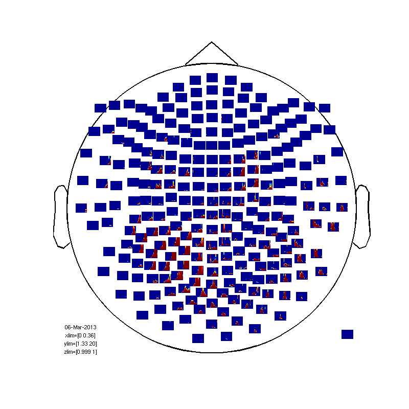
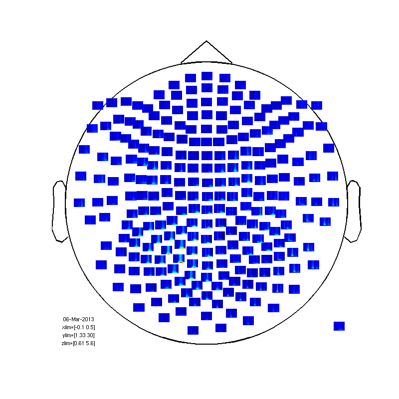
baseline=mean(TFrAll.powspctrm(:,:,:,1:6),4);
for timei=2:31;
    TFrAll.powspctrm(:,:,:,timei)=TFrAll.powspctrm(:,:,:,timei)-baseline;
end
% no compute the statistic
cfg=[];
cfg.method='stats';
nsubj=size(TFrAll.powspctrm,1);
cfg.design(1,:) = [ones(1,nsubj)];
cfg.latency     = [0 0.35];
cfg.frequency   = [1 20];
cfg.statistic = 'ttest'; % compares the mean to zero
cfg.feedback='no';
frstat=ft_freqstatistics(cfg,TFrAll);
% now plot 1-probability (1 = sig, less than 0.95 not sig)
cfg=[];
cfg.layout='4D248.lay';
frstat.powspctrm=1-frstat.prob;
cfg.zlim=[0.999 1]
cfg.interactive='yes';
fig3=figure;
set(fig3,'Position',[0,0,800,800]);
ft_multiplotTFR(cfg, frstat);

computing statistic over the frequency range [1.333 20.000]
computing statistic over the time range [0.000 0.350]
selection powspctrm along dimension 2
selection powspctrm along dimension 3
selection powspctrm along dimension 4
using "statistics_stats" for the statistical testing
number of observations 94240
number of replications 144
the call to "ft_freqstatistics" took 27 seconds and an estimated 207 MB

cfg = 

    layout: '4D248.lay'
      zlim: [0.9990 1]

reading layout from file 4D248.lay
the call to "ft_prepare_layout" took 0 seconds and an estimated 207 MB
Warning: (one of the) axis is/are not evenly spaced, but plots are made as if axis are linear 
the call to "ft_multiplotTFR" took 1 seconds and an estimated 207 MB